Gauss curvature approximation on embedded surfaces
In the previous notebook, we presented and discussed the distributional Gauss curvature and its lifting on Riemannian manifolds. However, we can also apply the method of high-order Gauss curvature on a surface \(\mathcal{S}\) embedded in \(\mathbb{R}^3\) with only a few adaptions of the method. Note that the theory can partly be extended from Riemannian manifolds to surfaces.
Setting
The surface can be expressed by its embedding \(\Phi\), which is a polynomial. If piecewise linear, we obtain a linear/affine approximation of the exact surface. If it is of higher order, the discrete geometry gets curved for better approximation. From \(\Phi\) we can compute its gradient \(F=\nabla \Phi\in \mathbb{R}^{3\times 2}\) and the metric tensor induced by the embedding via \(g= F^TF\in \mathbb{R}^{2\times 2}\). Note that the polynomial degree of \(g\) is \(2(k-1)\) if \(k\) is the order of the embedding \(\Phi\). Although the theory is available for such a \(g\), we won’t use a discrete lifted Gauss curvature of order \(2(k-1)+1\) to fit the theory, but the more natural choice of order \(k\). Furthermore, to make use of the theory that for a discrete metric stemming from the canonical Regge interpolant, we would need a commuting property of the form \(\mathcal{I}^{\mathrm{Reg}^{2(k-1)}}(g)= (\nabla \mathcal{I}^{\mathrm{Lag}^k}\Phi)^T(\nabla \mathcal{I}^{\mathrm{Lag}^k}\Phi)\), which in general does not hold.
Let \(\mathcal{S}\) be a surface with triangulation \(\mathcal{T}_h\). The finite element method to approximate the Gauss curvature reads: Find \(K_h \in V_h^k\) (the Lagrange finite element space of degree \(k\)) such that for all \(\varphi \in V_h^k\),
Here \(K|_T\) is the Gauss curvature in the interior of a triangle \(T\), \([\![\kappa_g]\!]\) is the jump of the geodesic curvature \(\kappa_g = \mu \cdot \nabla_t t\) across the edge \(E\), and
denotes the angle defect at the vertex \(V\).
Numerical example
[1]:
from ngsolve import *
from netgen.occ import *
from ngsolve.webgui import Draw
import random as random
from ngsolve.krylovspace import CGSolver
We define a function that computes the \(H^{-1}\)-norm of a functional \(f\), using the fact that \(||f||_{H^{-1}}\) is equivalent to \(\|u\|_{H^1}\) if \(-\Delta u = f\). We will use this function later to compute the error in the discrete Gauss curvature.
[2]:
# H^-1 norm
def ComputeHm1Norm(rhs, order):
fesH = H1(mesh, order=order)
u, v = fesH.TnT()
a = BilinearForm(
(Grad(u).Trace() * Grad(v).Trace() + u * v) * ds,
symmetric=True,
symmetric_storage=True,
condense=True,
)
f = LinearForm(rhs * v * ds).Assemble()
apre = Preconditioner(a, "bddc")
a.Assemble()
invS = CGSolver(a.mat, apre.mat, printrates="\r", maxiter=400)
ext = IdentityMatrix() + a.harmonic_extension
inv = a.inner_solve + ext @ invS @ ext.T
gfu = GridFunction(fesH)
gfu.vec.data = inv * f.vec
err = sqrt(Integrate(gfu**2 + Grad(gfu) ** 2, mesh, BND))
return err
Next we define a function that computes \(K_h = \sum_i u_i \varphi_i\) by solving the linear system \(Mu=f\), where \(M_{ij} = \int_{\mathcal{T}_h} \varphi_i \varphi_j da\) and
After computing \(K_h\), the function outputs the errors \(||K_h-K||_{H^{-1}}\) and \(||K_h-K||_{L^2}\).
[3]:
def ComputeGaussCurvature(mesh, order, Kex):
fes = H1(mesh, order=order)
u, v = fes.TnT()
# for angle deficit
bbnd_tang = specialcf.VertexTangentialVectors(3)
bbnd_tang1 = bbnd_tang[:, 0]
bbnd_tang2 = bbnd_tang[:, 1]
# for geodesic curvature
mu = Cross(specialcf.normal(3), specialcf.tangential(3))
edge_curve = specialcf.EdgeCurvature(3) # nabla_t t
# for elementwise Gauss curvature
def GaussCurvature():
nsurf = specialcf.normal(3)
return Cof(Grad(nsurf)) * nsurf * nsurf
# distributional Gauss curvature
f = LinearForm(fes)
# elementwise Gauss curvature
f += GaussCurvature() * v * ds
# jump of geodesic curvature
f += -edge_curve * mu * v * ds(element_boundary=True)
# one part of angle defect
f += -v * acos(bbnd_tang1 * bbnd_tang2) * ds(element_vb=BBND)
# mass matrix to compute discrete L2 Riesz representative
M = BilinearForm(u * v * ds, symmetric=True, symmetric_storage=True, condense=True)
gf_K = GridFunction(fes)
f.Assemble()
# second part of angle deficit (closed surface, no boundary)
for i in range(mesh.nv):
f.vec[i] += 2 * pi
Mpre = Preconditioner(M, "bddc")
M.Assemble()
invS = CGSolver(M.mat, Mpre.mat, printrates="\r", maxiter=400)
ext = IdentityMatrix() + M.harmonic_extension
inv = M.inner_solve + ext @ invS @ ext.T
gf_K.vec.data = inv * f.vec
l2_err = sqrt(Integrate((gf_K - Kex) ** 2, mesh, BND))
hm1_err = ComputeHm1Norm(gf_K - Kex, order=order + 2)
print(
f" Check Gauss-Bonnet theorem: int gf_K = {Integrate(gf_K * ds(bonus_intorder=5), mesh)}"
f" = 4*pi = {4 * pi}"
)
# uncomment to draw Gauss curvature
Draw(gf_K, mesh, "K")
return l2_err, hm1_err, fes.ndof
Now, we are ready to test the method. We triangulate an ellipsoid (using curved triangles of a given order), compute the Gaussian curvature, measure the error, and repeat several refinements. We also check how well the lifted Gauss curvature fulfils the Gauss-Bonnet theorem \(\int_{\mathcal{T}_h}K_h\,da = 2\pi\chi(\mathcal{S}) = 4\pi\).
[4]:
order = 1
# radius of sphere/ellipsoid
R = 3
# use sphere or ellipsoid surface
if False: # sphere
geo = Sphere((0, 0, 0), R).faces[0]
# exact Gauss curvature of sphere
Kex = 1 / R**2
else: # ellipsoid
a = R
b = R
c = 3 / 4 * R
geo = Ellipsoid(Axes((0, 0, 0), X, Y), a, b, c).faces[0]
# exact Gauss curvature of ellipsoid
Kex = 1 / (a**2 * b**2 * c**2 * (x**2 / a**4 + y**2 / b**4 + z**2 / c**4) ** 2)
err_l2 = []
err_hm1 = []
ndof = []
with TaskManager():
for i in range(4 + (order == 1)):
mesh = Mesh(OCCGeometry(geo).GenerateMesh(maxh=0.5**i)).Curve(order)
errl, errm1, dof = ComputeGaussCurvature(mesh, order, Kex=Kex)
err_l2.append(errl)
err_hm1.append(errm1)
ndof.append(dof)
CG converged in 2 iterations to residual 4.530232866875219e-16
CG converged in 10 iterations to residual 1.6675010826207632e-14
Check Gauss-Bonnet theorem: int gf_K = 12.566370614358728 = 4*pi = 12.566370614359172
CG converged in 2 iterations to residual 3.3314159843685105e-16
CG converged in 11 iterations to residual 3.842523892768551e-15
Check Gauss-Bonnet theorem: int gf_K = 12.566370614359519 = 4*pi = 12.566370614359172
CG converged in 2 iterations to residual 4.584368956308179e-16
CG converged in 11 iterations to residual 4.419424413736214e-15
Check Gauss-Bonnet theorem: int gf_K = 12.566370614360908 = 4*pi = 12.566370614359172
CG converged in 2 iterations to residual 3.8224146081100207e-16
CG converged in 12 iterations to residual 2.22631782752086e-16
Check Gauss-Bonnet theorem: int gf_K = 12.566370614358839 = 4*pi = 12.566370614359172
CG converged in 2 iterations to residual 6.877006100331674e-16
CG converged in 12 iterations to residual 3.626850358389609e-16
Check Gauss-Bonnet theorem: int gf_K = 12.566370614372078 = 4*pi = 12.566370614359172
Finally, we plot the errors against the number of degrees of freedom.
[5]:
import matplotlib.pyplot as plt
plt.plot(ndof, err_hm1, "-o", label=r"$\|K_h-K_{\mathrm{ex}}\|_{H^{-1}}$")
plt.plot(ndof, err_l2, "-x", label=r"$\|K_h-K_{\mathrm{ex}}\|_{L^2}$")
plt.plot(
ndof,
[order**order * dof ** (-(order - 1) / 2) for dof in ndof],
"-.",
color="k",
label=f"$O(h^{order - 1})$",
)
plt.plot(
ndof,
[order**order * dof ** (-(order) / 2) for dof in ndof],
"-",
color="k",
label=f"$O(h^{order})$",
)
plt.plot(
ndof,
[order**order * dof ** (-(order + 1) / 2) for dof in ndof],
"--",
color="k",
label=f"$O(h^{order + 1})$",
)
plt.yscale("log")
plt.xscale("log")
plt.legend()
plt.title(f"order = {order}")
plt.show()
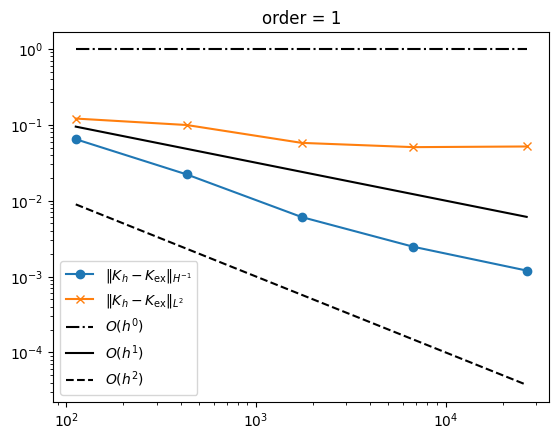
Observations: Except for \(k=2\), we observe the convergence rates
One additional order of convergence is observed for \(k=2\) of curving the surface quadratically. This could be a lucky case where the theory of improved convergence rates applies.
[ ]: