Distributional Einstein curvature
This notebook discusses the definition and convergence of the distributional Einstein tensor in dimensions three and higher (in one and two dimensions, the Einstein tensor is zero). For a detailed derivation and analysis, we refer to Gawlik, Neunteufel. Finite element approximation of the Einstein tensor, IMA Journal of Numerical Analysis (2025)..
Einstein tensor as a nonlinear distribution
The Einstein tensor reads with the Ricci curvature tensor \(\mathrm{Ric}\) and scalar curvature \(S\) \begin{align*} G = \mathrm{Ric}-\frac{1}{2}S\,g. \end{align*} One important application of the Einstein tensor for pseudo-Riemannian manifolds is general relativity. The Einstein field equations \(G=8\pi\mathfrak{T}\), where \(\mathfrak{T}\) is the energy-stress tensor, describe cosmologic phenomena such as black holes.
Motivated by the integral representation of the distributional scalar curvature, we define the distributional (densitized) Einstein tensor acting on a sufficiently smooth matrix-valued test function \(\varphi\) as
where \(\omega_T\), \(\omega_F\), and \(\omega_E\) are the respective volume forms on elements \(T\), co-dimension 1 facets \(F\) and co-dimension two boundaries \(E\). \(\bar{I\!I}=I\!I-H\,g\) is the trace-reversed second fundamental form with mean curvature \(H\)
where \(n\) is the normal vector at the facet (caution: Different sign conventions exist again). \(\Theta_E\) is the angle defect. As we have seen in the previous notebook, the concept of the angle defect directly extends from 2D to any dimension.
The jump of the trace-reversed second fundamental form at facets is well-known in physics literature as the Israel junction conditions Israel. Singular hypersurfaces and thin shells in general relativity, Nuovo Cimento B (1965-1970) 1966. verifying our distributional facet term.
Integral representation and convergence
The distributional EInstein tensor entails an integral representation, which is more involved than the scalar curvature. Taking the variation of the densitized distributional Einstein tensor in the metric in direction \(\sigma\) yields
with
Here, all differential operators are covariant ones with respect to the metric \(g\), and \(\nu\) denotes the co-normal vector being perpendicular to the co-dimension 2 boundary \(E\) pointing from \(E\) into the adjacent facets \(F\) of the element \(T\). \(\mathrm{ein}\) is the (covariant) linearized Einstein operator defined by
and \(\mathbb{S}_F\sigma=\sigma|_F-\mathrm{tr}(\sigma|_F)g|_F\). Note that \(A(g;\sigma,\rho)\) and \(B(g;\sigma,\rho)\) become identically zero in two dimensions. \(B_h(g;\sigma,\rho)\) can be interpreted as a distributional (covariant) extension of the linearized Einstein operator \(\mathrm{ein}\) for tangential-tangential continuous matrices. In three dimensions, the linearized Einstein operator coincides with the incompatibility operator by up to a factor of \(2\).
The convergence rates in the \(H^{-2}\) norm for \(k\ge 0\) and \(g_h\in \mathrm{Reg}^k\) coincide with those of the distributional scalar curvature
Again, we cannot expect convergence in the lowest-order case of a piecewise constant Regge metric. When going to linear order, the convergence rate jumps to be quadratic. Then, the dependency on the polynomial approximation order relates to the convergence rate as expected.
Numerical example
In the following example, we compute the distributional Einstein tensor \(\widetilde{G\omega}\) on a sequence of meshes for a three-dimensional Riemannian manifold and compute the \(H^{-2}\) error.
[1]:
from ngsolve.meshes import MakeStructured3DMesh
from ngsolve import *
from ngsolve.webgui import Draw
import random as random
from ngsolve.krylovspace import CGSolver
import numpy as np


def mapping(x, y, z):
    return (2 * x - 1, 2 * y - 1, 2 * z - 1)


mesh = MakeStructured3DMesh(False, nx=12, ny=12, nz=12, mapping=mapping)

peak = (
    0.5 * x**2 - 1 / 12 * x**4 + 0.5 * y**2 - 1 / 12 * y**4 + 0.5 * z**2 - 1 / 12 * z**4
)

F = CF(
    (1, 0, 0, 0, 1, 0, 0, 0, 1, peak.Diff(x), peak.Diff(y), peak.Diff(z)), dims=(4, 3)
)
G_ex = F.trans * F


def q(X):
    return X**2 * (X**2 - 3) ** 2


# exact Ricci curvature tensor
Ricci11 = (
    -9
    * (x**2 - 1)
    * ((y**2 + z**2 - 2) * (q(x) + 9) + (z**2 - 1) * q(y) + q(z) * (y**2 - 1))
    / (9 + q(x) + q(y) + q(z)) ** 2
)
Ricci22 = (
    -9
    * (y**2 - 1)
    * ((x**2 + z**2 - 2) * (q(y) + 9) + (z**2 - 1) * q(x) + q(z) * (x**2 - 1))
    / (9 + q(x) + q(y) + q(z)) ** 2
)
Ricci33 = (
    -9
    * (z**2 - 1)
    * ((y**2 + x**2 - 2) * (q(z) + 9) + (x**2 - 1) * q(y) + q(x) * (y**2 - 1))
    / (9 + q(x) + q(y) + q(z)) ** 2
)
Ricci12 = (
    -9
    * (y**2 - 3)
    * y
    * (x**2 - 3)
    * x
    * (x**2 - 1)
    * (y**2 - 1)
    / (9 + q(x) + q(y) + q(z)) ** 2
)
Ricci13 = (
    -9
    * (z**2 - 3)
    * z
    * (x**2 - 3)
    * x
    * (x**2 - 1)
    * (z**2 - 1)
    / (9 + q(x) + q(y) + q(z)) ** 2
)
Ricci23 = (
    -9
    * (y**2 - 3)
    * y
    * (z**2 - 3)
    * z
    * (z**2 - 1)
    * (y**2 - 1)
    / (9 + q(x) + q(y) + q(z)) ** 2
)

Ricci_ex = -CF(
    (Ricci11, Ricci12, Ricci13, Ricci12, Ricci22, Ricci23, Ricci13, Ricci23, Ricci33),
    dims=(3, 3),
)

# exact scalar curvature
S_ex = (
    -(
        2 * ((1 - z**2) * y**2 + z**2 - 1) * x**12
        + 24 * ((-1 + z**2) * y**2 - z**2 + 1) * x**10
        + (
            2 * (1 - z**2) * y**6
            + 12 * (-1 + z**2) * y**4
            + (108 - 2 * z**6 - 144 * z**2 + 12 * z**4) * y**2
            - 72
            - 12 * z**4
            + 108 * z**2
            + 2 * z**6
        )
        * x**8
        + (
            2 * (1 - z**2) * y**8
            + 28 * (-1 + z**2) * y**6
            + 114 * (1 - z**2) * y**4
            + (468 * z**2 + 28 * z**6 - 2 * z**8 - 198 - 114 * z**4) * y**2
            - 72
            + 114 * z**4
            + 2 * z**8
            - 28 * z**6
            - 198 * z**2
        )
        * x**6
        + (
            (-12 + 12 * z**2) * y**8
            + (114 - 114 * z**2) * y**6
            + (-360 + 360 * z**2) * y**4
            + (360 * z**4 - 114 * z**6 + 12 * z**8 + 54 - 702 * z**2) * y**2
            + 594
            + 114 * z**6
            - 12 * z**8
            - 360 * z**4
            + 54 * z**2
        )
        * x**4
        + (
            (2 - 2 * z**2) * y**12
            + (-24 + 24 * z**2) * y**10
            + (108 - 2 * z**6 - 144 * z**2 + 12 * z**4) * y**8
            + (468 * z**2 + 28 * z**6 - 2 * z**8 - 198 - 114 * z**4) * y**6
            + (360 * z**4 - 114 * z**6 + 12 * z**8 + 54 - 702 * z**2) * y**4
            + (486 + 468 * z**6 - 2 * z**12 + 24 * z**10 - 144 * z**8 - 702 * z**4)
            * y**2
            + 108 * z**8
            - 324
            - 24 * z**10
            + 2 * z**12
            - 198 * z**6
            + 54 * z**4
            + 486 * z**2
        )
        * x**2
        + (2 * z**2 - 2) * y**12
        + (-24 * z**2 + 24) * y**10
        + (-72 - 12 * z**4 + 108 * z**2 + 2 * z**6) * y**8
        + (-72 + 114 * z**4 + 2 * z**8 - 28 * z**6 - 198 * z**2) * y**6
        + (594 + 114 * z**6 - 12 * z**8 - 360 * z**4 + 54 * z**2) * y**4
        + (
            108 * z**8
            - 324
            - 24 * z**10
            + 2 * z**12
            - 198 * z**6
            + 54 * z**4
            + 486 * z**2
        )
        * y**2
        - 486
        - 72 * z**8
        + 24 * z**10
        - 2 * z**12
        - 72 * z**6
        + 594 * z**4
        - 324 * z**2
    )
    / (
        1
        + 1 / 9 * x**6
        + 1 / 9 * y**6
        + 1 / 9 * z**6
        - 2 / 3 * y**4
        + y**2
        - 2 / 3 * x**4
        + x**2
        - 2 / 3 * z**4
        + z**2
    )
    / (
        x**6
        + y**6
        + z**6
        - 6 * x**4
        - 6 * y**4
        - 6 * z**4
        + 9 * x**2
        + 9 * y**2
        + 9 * z**2
        + 9
    )
    ** 2
)

# exact Einstein tensor
Einstein_ex = Ricci_ex - 1 / 2 * S_ex * G_ex
clipping = {"pnt": (0, 0, 0.01), "z": -1, "function": True}
Draw(Norm(Einstein_ex), mesh, clipping=clipping);
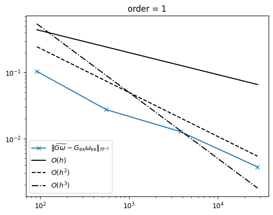
We compute the \(H^{-2}\)-norm of the error \(\|\widetilde{G\omega}-G\omega\|_{H^{-2}}\) by solving for each component the following fourth-order problem \(\mathrm{div}(\mathrm{div}(\nabla^2 u_{ij}))= (\widetilde{G\omega}-G\omega)_{ij}\). Then \(\|u\|_{H^2}\approx \|\widetilde{G\omega}-G\omega\|_{H^{-2}}\). We use the Euclidean Hellan-Herrmann-Johnson (HHJ) method to solve the fourth-order problem as a mixed saddle point problem. Therein, \(\sigma=\nabla^2u_{ij}\) is introduced as an additional unknown. We use hybridization techniques to regain a minimization problem. We use a BDDC preconditioner in combination with static condensation and a CGSolver to solve the problem iteratively. To mitigate approximation errors that spoil the convergence, we use two polynomial degrees more than for \(g_h\) to compute \(u_h\).
[2]:
def ComputeHm2Norm(func_vol, func_bnd, func_bbnd, mesh, order):
    fesH = H1(mesh, order=order, dirichlet=".*")
    fesS = Discontinuous(HDivDiv(mesh, order=order - 1))
    fesHB = NormalFacetFESpace(mesh, order=order - 1, dirichlet=".*")
    fes = fesH * fesS * fesHB
    (u, sigma, uh), (v, tau, vh) = fes.TnT()

    n = specialcf.normal(mesh.dim)

    a = BilinearForm(fes, symmetric=True, symmetric_storage=True, condense=True)
    a += (
        InnerProduct(sigma, tau)
        - InnerProduct(tau, u.Operator("hesse"))
        - InnerProduct(sigma, v.Operator("hesse"))
    ) * dx
    a += ((Grad(u) - uh) * n * tau[n, n] + (Grad(v) - vh) * n * sigma[n, n]) * dx(
        element_boundary=True
    )

    apre = Preconditioner(a, "bddc")
    a.Assemble()

    invS = CGSolver(a.mat, apre, printrates="\r", maxiter=600)
    if a.condense:
        ext = IdentityMatrix() + a.harmonic_extension
        inv = a.inner_solve + ext @ invS @ ext.T
    else:
        inv = invS

    # use MultiVector to solve for all right-hand sides at once
    rhs = MultiVector(fes.ndof, 6, False)
    gf_u_i = GridFunction(fes**6)

    for i in range(6):
        j = i if i < 3 else (i + 1 if i < 5 else 8)
        f = LinearForm(
            func_vol[j] * v * dx
            + func_bnd[j] * v * dx(element_boundary=True)
            + func_bbnd[j] * v * dx(element_vb=BBND)
        )
        f.Assemble()
        rhs[i].data = f.vec

    gfu_multivec = (inv * rhs).Evaluate()

    for i in range(6):
        gf_u_i.components[i].vec.data = gfu_multivec[i]

    index_symmetric_matrix = [0, 1, 2, 1, 3, 4, 2, 4, 5]
    # u
    gfu = CF(
        tuple([gf_u_i.components[i].components[0] for i in index_symmetric_matrix]),
        dims=(3, 3),
    )
    # Grad(u)
    grad_gfu = CF(
        tuple(
            [Grad(gf_u_i.components[i].components[0]) for i in index_symmetric_matrix]
        ),
        dims=(3, 3, 3),
    )
    # sigma = hesse u
    gf_sigma = CF(
        tuple([gf_u_i.components[i].components[1]] for i in index_symmetric_matrix),
        dims=(3, 3, 3, 3),
    )
    err = sqrt(
        Integrate(
            InnerProduct(gfu, gfu)
            + InnerProduct(grad_gfu, grad_gfu)
            + InnerProduct(gf_sigma, gf_sigma),
            mesh,
        )
    )
    return err
The following function computes the \(H^2\)-error of the distributional Einstein tensor for a given metric and polynomial order.
[3]:
def ComputeEinsteinCurvature(mesh, G, order):
    bbnd_tang = specialcf.EdgeFaceTangentialVectors(3)
    tE = specialcf.tangential(mesh.dim, True)
    tef1 = bbnd_tang[:, 0]
    tef2 = bbnd_tang[:, 1]
    n1 = Cross(tef1, tE)
    n2 = Cross(tef2, tE)
    n = specialcf.normal(mesh.dim)

    # Regge metric
    fesCC = HCurlCurl(mesh, order=order)
    gfG = GridFunction(fesCC)
    gfG.Set(G)

    # volume forms
    vol_bbnd = sqrt(gfG * tE * tE)
    vol_bnd = sqrt(Cof(gfG) * n * n)
    vol = sqrt(Det(gfG))

    # co-dimension 2 term
    n1g = 1 / sqrt(Inv(gfG) * n1 * n1) * Inv(gfG) * n1
    n2g = 1 / sqrt(Inv(gfG) * n2 * n2) * Inv(gfG) * n2
    tEg = 1 / sqrt(gfG * tE * tE) * tE
    func_bbnd = (
        -vol_bbnd * (acos(n1 * n2) - acos(gfG * n1g * n2g)) * OuterProduct(tEg, tEg)
    )

    # co-dimension 1 facet term
    ng = 1 / sqrt(Inv(gfG) * n * n) * Inv(gfG) * n
    SFF = -gfG.Operator("christoffel") * ng
    P = Inv(gfG) - OuterProduct(ng, ng)
    H = InnerProduct(gfG, P * SFF * P)
    func_bnd = vol_bnd * P * (SFF - H * gfG) * P

    # volume term
    func_vol = vol * Inv(gfG) * gfG.Operator("Einstein") * Inv(gfG) - sqrt(
        Det(G_ex)
    ) * (Inv(G_ex) * Einstein_ex * Inv(G_ex))

    err_hm2 = ComputeHm2Norm(func_vol, func_bnd, func_bbnd, mesh, order=order + 2)

    return (err_hm2, fesCC.ndof)
To avoid possible super-convergence due to symmetries in the mesh, we perturb the internal vertices by a random noise.
[4]:
# compute the diameter of the mesh as maximal mesh size h
def CompDiam(mesh):
    lengths = np.zeros(mesh.nedge)
    for edge in mesh.edges:
        pnts = []
        for vert in edge.vertices:
            pnt = mesh[vert].point
            pnts.append((pnt[0], pnt[1], pnt[2]))
        lengths[edge.nr] = sqrt(
            (pnts[0][0] - pnts[1][0]) ** 2
            + (pnts[0][1] - pnts[1][1]) ** 2
            + (pnts[0][2] - pnts[1][2]) ** 2
        )

    print(f"max = {max(lengths)}, min = {min(lengths)}, ne = {mesh.ne}")
    return max(lengths)


# generate and randomly perturb it, check if the resulting mesh is valid
def GenerateRandomMesh(k, par):
    for i in range(20):
        mesh = MakeStructured3DMesh(False, nx=2**k, ny=2**k, nz=2**k, mapping=mapping)
        maxh = CompDiam(mesh)
        for pnts in mesh.ngmesh.Points():
            px, py, pz = pnts[0], pnts[1], pnts[2]
            if (
                abs(px + 1) > 1e-8
                and abs(px - 1) > 1e-8
                and abs(py + 1) > 1e-8
                and abs(py - 1) > 1e-8
                and abs(pz + 1) > 1e-8
                and abs(pz - 1) > 1e-8
            ):
                px += random.uniform(-maxh / 2**par / sqrt(2), maxh / 2**par / sqrt(2))
                py += random.uniform(-maxh / 2**par / sqrt(2), maxh / 2**par / sqrt(2))
                pz += random.uniform(-maxh / 2**par / sqrt(2), maxh / 2**par / sqrt(2))
            pnts[0] = px
            pnts[1] = py
            pnts[2] = pz
        F = specialcf.JacobianMatrix(3)
        # check if the mesh is valid
        if Integrate(IfPos(Det(F), 0, -1), mesh) >= 0:
            break
    else:
        raise Exception("Could not generate a valid mesh")

    return mesh
Compute the Einstein tensor approximation on a sequence of meshes. You can play around with the polynomial order. The \(H^{-2}\) error and the number of degrees of freedom are stored.
[5]:
err_hm2 = []
ndof = []

# order of metric approximation >= 0
order = 1

with TaskManager():
    for i in range(4):
        mesh = GenerateRandomMesh(k=i, par=3)
        errm2, dof = ComputeEinsteinCurvature(mesh, G=G_ex, order=order)
        err_hm2.append(errm2)
        ndof.append(dof)
max = 3.4641016151377544, min = 2.0, ne = 6
CG converged in 13 iterations to residual 8.100592550775689e-15
CG converged in 9 iterations to residual 3.0041599110386764e-14
CG converged in 10 iterations to residual 2.4778564957102608e-14
CG converged in 13 iterations to residual 7.779627351727951e-15
CG converged in 10 iterations to residual 2.112658322912368e-14
CG converged in 13 iterations to residual 7.901458615975567e-15
max = 1.7320508075688772, min = 1.0, ne = 48
CG converged in 36 iterations to residual 8.951282028095007e-15
CG converged in 35 iterations to residual 6.040638932001146e-15
CG converged in 36 iterations to residual 2.8003619507917304e-15
CG converged in 36 iterations to residual 9.150789829408781e-15
CG converged in 36 iterations to residual 2.806918032537161e-15
CG converged in 35 iterations to residual 1.9721225519961012e-14
max = 0.8660254037844386, min = 0.5, ne = 384
CG converged in 57 iterations to residual 9.486811637376685e-15
CG converged in 57 iterations to residual 3.100742801216868e-15
CG converged in 57 iterations to residual 3.1454247850621556e-15
CG converged in 58 iterations to residual 6.733601945931407e-15
CG converged in 57 iterations to residual 4.234006442187017e-15
CG converged in 57 iterations to residual 8.051988887420032e-15
max = 0.4330127018922193, min = 0.25, ne = 3072
CG converged in 63 iterations to residual 2.86825761741079e-15
CG converged in 63 iterations to residual 1.108379392991975e-15
CG converged in 63 iterations to residual 1.1360607720450064e-15
CG converged in 63 iterations to residual 2.8544568976083382e-15
CG converged in 63 iterations to residual 1.1330465366603615e-15
CG converged in 63 iterations to residual 2.790143976374909e-15
Plot the results together with reference lines for linear, quadratic, and cubic convergence order.
[6]:
import matplotlib.pyplot as plt

plt.plot(
    ndof,
    err_hm2,
    "-x",
    label=r"$\|\widetilde{G\omega}-G_{\mathrm{ex}}\omega_{\mathrm{ex}}\|_{H^{-2}}$",
)
plt.plot(ndof, [2 * dof ** (-1 / 3) for dof in ndof], "-", color="k", label="$O(h)$")
plt.plot(ndof, [5 * dof ** (-2 / 3) for dof in ndof], "--", color="k", label="$O(h^2)$")
plt.plot(
    ndof, [50 * dof ** (-3 / 3) for dof in ndof], "-.", color="k", label="$O(h^3)$"
)


plt.yscale("log")
plt.xscale("log")
plt.legend()
plt.title(f"order = {order}")
plt.show()
[ ]: