Distributional Riemann curvature tensor

In this notebook, we discuss the distributional Riemann curvature tensor in arbitrary dimensions. The Riemann curvature tensor stores all the information about the curvature of a Riemannian manifold. From it, we can compute all other curvature quantities, such as the Ricci and Einstein tensor, and the scalar and (in 2D) the Gauss curvature. This also answers the following fundamental question positively: Is it possible to define all intrinsic curvature quantities from a Regge metric? For a detailed derivation and analysis, we refer to Gopalakrishnan, Neunteufel, Schöberl, Wardetzky. Generalizing Riemann curvature to Regge metrics, arXiv (2024)..

Riemann curvature tensor as a nonlinear distribution

The Riemann curvature tensor is a fourth-order tensor with several (skew)-symmetry properties. The distributional (densitized) Riemann curvature tensor acting on specific tensor-valued test functions \(A\in\mathcal{A}\) is defined as

\[\begin{align*} \widetilde{\mathfrak{R}\omega}(A) :=\sum_{T\in\mathcal{T}}\int_T\langle \mathfrak{R}|_T,A\rangle\,\omega_T+4\sum_{F\in\mathcal{F}}\int_F\langle[\![I\!I]\!],A(\cdot,\nu,\nu,\cdot)\rangle\,\omega_F+4\sum_{E\in\mathcal{E}}\int_E\Theta_E\,A(\mu,\nu,\nu,\mu)\,\omega_E, \end{align*}\]

where \(\omega_T\), \(\omega_F\), and \(\omega_E\) are the respective volume forms on elements \(T\), co-dimension 1 facets \(F\) and co-dimension two boundaries \(E\). \(I\!I\) denotes the second fundamental form

\[\begin{align*} I\!I(X,Y) = -g(\nabla_X\nu,Y)=g(\nabla_XY,\nu),\quad X,Y\in \mathfrak{X}(F), \end{align*}\]

Here \(\nu\) is the inward unit normal of each element at the facet, as in the paper and the numerical example’s normal_sign=-1. Writing \(n=-\nu\) for the outward normal gives \(I\!I(X,Y)=g(\nabla_Xn,Y)\), the convention used in the scalar-curvature and Einstein-tensor notebooks. \(\Theta_E\) is the angle defect and \(\mu\) the co-normal vector being \(g\)-perpendicular to the co-dimension 2 boundary \(E\) and pointing from \(E\) into the element \(T\) along one of the facets \(F\) adjacent to \(E\). The test functions entail the same symmetry properties as the Riemann curvature tensor and have to fulfil the following continuity requirement at internal facets \(F\)

\[\begin{align*} A(\cdot,\nu,\nu,\cdot) \text{ is single valued for all $F\in\mathcal{F}$, i.e. } [\![A(\cdot,\nu,\nu,\cdot)]\!]_F=0. \end{align*}\]

From it, we can prove that \(A(\mu,\nu,\nu,\mu)\) is single-valued at all co-dimension 2 boundaries \(E\).

A heuristic motivation of the jump of the second fundamental form as the facet is given as follows: Consider a facet \(F\) that is a subsimplex of two adjacent elements \(T_\pm\) with respective unit normal vectors \(\nu_\pm\) at a point \(p\) in \(F\). Also consider two \(2\)-dimensional submanifolds \(S_\pm\) of \(T_\pm\) passing through \(p\) and transversely intersecting \(F\) along a smooth curve \(\gamma\) in \(F\), such that one tangent direction at \(p\) is parallel to the respective normal \(\nu_{\pm}\). Denote the unit tangent vector along \(\gamma\) at \(p\) by \(X\). Let \(\mathfrak{R}_\pm\) be the respective Riemann curvature tensors of \(T_\pm\). The respective sectional curvatures at \(p\) generated by the orthonormal pair \(X, \nu_\pm\) equal \(\mathfrak{R}_\pm(X, \nu_\pm, \nu_\pm, X)\). It is well-known that these sectional curvatures coincide with the Gauss curvatures of \(S_\pm\). Since we know that the distributional Gauss curvature of the composite \(2\)-manifold \(S_+ \cup S_-\) must have an interface curvature contribution arising from the jump of the geodesic curvatures \(\kappa_\pm \equiv I\!I_\pm(X, X)\) from adjacent elements, we conclude that the difference between \(\mathfrak{R}_\pm(X, \nu_\pm, \nu_\pm, X)\) at \(p\) must equal the difference between \(I\!I_+(X, X)\) and \(I\!I_-(X, X)\). This result can be extended to any \(X\) in the tangent space of \(F\) at \(p\) by varying the 2-manifold. Furthermore, by the symmetry of \(\mathfrak{R}_\pm(X, \nu_\pm, \nu_\pm, Y)\) in \(X\) and \(Y\), the polarization identity implies that the jump of \(\mathfrak{R}_\pm(X, \nu_\pm, \nu_\pm, Y)\) must equal the jump of \(I\!I_\pm(X, Y)\) for any \(X, Y\) in the tangent space of \(F\).

Integral representation and convergence

The distributional Riemann curvature tensor entails an integral representation, which is crucial for numerical analysis. The test function space \(\mathcal{A}\) depends on the metric \(g\). The Uhlenbeck trick maps a fixed, metric-independent test tensor \(U\) to \(A_U(g)\in\mathcal{A}(g)\); the variation below holds \(U\) fixed and differentiates \(A_U(g)\) along with the curvature functional. We skip the details and present the final integral representation.

Taking the variation of the densitized distributional Riemann curvature tensor in the metric in direction \(\sigma\) yields

\[\begin{align*} \left.\frac{d}{dt}\widetilde{\mathfrak{R}\omega}_{g(t)}(A_U(g(t)))\right|_{t=0} = a_h(g;\sigma,A_U)+b_h(g;\sigma,A_U),\qquad \sigma=\dot g(0), \end{align*}\]

with

\[\begin{split}\begin{align*} a_h(g;\sigma,A)&= \sum_T\int_T\left(\langle L_{\sigma}^{(1)}\mathfrak{R},A\rangle-\frac12\mathrm{tr}_g(\sigma)\langle\mathfrak{R},A\rangle\right)\,\omega_T\\ &\quad+2\sum_F\int_F [\![I\!I]\!]_F:\mathbb{S}_F(\sigma):A(\cdot,\nu,\nu,\cdot)\,\omega_F\\ &\quad-2\sum_{E}\int_E\mathrm{tr}(\sigma_E)\,\Theta_E\,A(\mu,\nu,\nu,\mu)\,\omega_E,\\ b_h(g;\sigma,A)&= 2\sum_T\int_T\langle\nabla^2\sigma,SA\rangle\,\omega_T\\ &\quad+2\sum_F\int_F\left\langle[\![\sigma(\nu,\nu)I\!I+(\nabla\sigma)_{F\nu F}+(\nabla(\nu\mathbin{\lrcorner}\sigma))_F-(\nabla\sigma)_{\nu FF}]\!],A(\cdot,\nu,\nu,\cdot)\right\rangle\,\omega_F\\ &\quad-2\sum_E\int_E\sum_{F\supset E}[\![\sigma(\mu,\nu)]\!]_F^E A(\mu,\nu,\nu,\mu)\,\omega_E. \end{align*}\end{split}\]

Here, all differential operators are covariant ones with respect to the metric \(g\). Further, \(\mathbb{S}_F(\sigma)=\sigma|_F-\mathrm{tr}(\sigma|_F)g_F\), \((SA)(X,Y,Z,W) =A(X,Z,Y,W)\), and \((L_{\sigma}^{(1)}\mathfrak{R})(X,Y,Z,W) =\mathfrak{R}(L_{\sigma}X,Y,Z,W)\) with \(L_{\sigma}\) the endomorphism defined by \(g(L_{\sigma}X,Y) = \sigma(X,Y)\). Due to the skew-symmetry of \(SA\), the bilinear form \(b_h(g;\sigma,A)\) can be interpreted as a distributional covariant extension of the incompatibility operator in arbitrary dimensions.

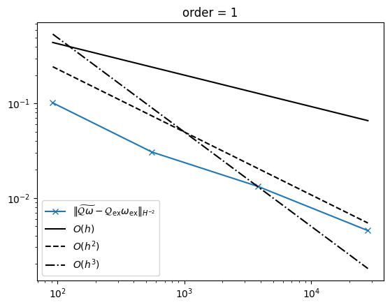
As expected, we obtain the same convergence rates as for the distributional scalar curvature in the \(H^{-2}\) norm for \(k\ge 0\) and \(g_h\in \mathrm{Reg}^k\)

\[\begin{split}\begin{align*} \|\widetilde{\mathfrak{R}\omega}(g_h)-(\mathfrak{R}\omega)(g)\|_{H^{-2}}\le C\begin{cases} h^{k+1}, & N=2\\ h^{\min\{k+1,2k\}}, &N \ge 3 \end{cases}. \end{align*}\end{split}\]

Specialization in 3D

In three dimensions, we can use that the curvature operator \(\mathcal{Q}\) is related to the Riemann curvature operator via

\[\begin{align*} \mathcal{Q}(X\times Y, W\times Z) = \mathfrak{R}(X,Y,Z,W),\qquad \forall X,Y,Z,W\in \mathfrak{X}(M), \end{align*}\]

where \(X\times Y\) is the covariant cross product defined by \(\omega(X,Y,\cdot)^\sharp\). Further, there holds the following relation between the test functions \(A\in\mathcal{A}\) and the Regge function \(U\in\mathrm{Reg}\)

\[\begin{align*} A^{ijkl} = -\varepsilon^{ijm}\varepsilon^{kln}U_{mn}, \end{align*}\]

Here \(\widehat{\varepsilon}^{ijk}\) is the alternating symbol and \(\varepsilon^{ijk}=(\det g)^{-1/2}\widehat{\varepsilon}^{ijk}\) is the contravariant volume tensor. The minus sign follows from the order of the last two arguments of \(\mathfrak{R}(X,Y,Z,W)\): for \(g=I\) and \(U=e_3^\flat\otimes e_3^\flat\), one has \(A(e_1,e_2,e_2,e_1)=1\). Inserting into the definition of the distributional Riemann curvature tensor and simplifying yields the following distributional curvature operator

\[\begin{align*} \widetilde{{\mathcal{Q}}\omega}(U)=&\sum_{T\in\mathcal{T}}\int_T\langle {\mathcal{Q}}_T,U\rangle\,\omega_T+\sum_{F\in\mathcal{F}}\int_F\langle[\![I\!I]\!],(\nu^\flat\otimes\nu^\flat)\times U\rangle\,\omega_F+\sum_{E\in\mathcal{E}}\int_E \Theta_E\, U_{\tau_E\tau_E}\,\omega_E, \end{align*}\]

Here \(\tau_E\) is the \(g\)-unit tangent vector of the edge \(E\) and \((B\times C)^{ij}=\varepsilon^{ikl}\varepsilon^{jmn}B_{km}C_{ln}\) denotes the tensor cross product. Since \((\nu^\flat\otimes\nu^\flat)\times U=-\mathbb{S}_F U\), the facet term equals \(-\langle[\![\overline{I\!I}]\!],U_F\rangle\), as in the paper, where \(\overline{I\!I}=\mathbb{S}_F(I\!I)\). In three dimensions, \(\mathcal{Q}=-G^{\sharp\sharp}\) for the Riemann-tensor convention used here. We will use this expression for the numerical example.

Numerical example

In the following example, we compute the distributional Riemann curvature tensor \(\widetilde{\mathfrak{R}\omega}\), more precisely its equivalent curvature operator form \(\widetilde{\mathcal{Q}\omega}\), on a sequence of meshes for a three-dimensional Riemannian manifold and compute the \(H^{-2}\) error.

from ngsolve.meshes import MakeStructured3DMesh
from ngsolve import *
import ngsdiffgeo as dg
import random as random
from ngsolve.krylovspace import CGSolver
import numpy as np
from ngsolve.webgui import Draw


def mapping(x, y, z):
    return (2 * x - 1, 2 * y - 1, 2 * z - 1)


mesh = MakeStructured3DMesh(False, nx=6, ny=6, nz=6, mapping=mapping)


peak = (
    0.5 * x**2 - 1 / 12 * x**4 + 0.5 * y**2 - 1 / 12 * y**4 + 0.5 * z**2 - 1 / 12 * z**4
)

F = CF(
    (1, 0, 0, 0, 1, 0, 0, 0, 1, peak.Diff(x), peak.Diff(y), peak.Diff(z)), dims=(4, 3)
)
G_ex = F.trans * F


def q(x):
    return x**2 * (x**2 - 3) ** 2


Qex_xx = 9 * (z**2 - 1) * (y**2 - 1) / (q(x) + q(y) + q(z) + 9)
Qex_xy = 0
Qex_xz = 0
Qex_yy = 9 * (z**2 - 1) * (x**2 - 1) / (q(x) + q(y) + q(z) + 9)
Qex_yz = 0
Qex_zz = 9 * (y**2 - 1) * (x**2 - 1) / (q(x) + q(y) + q(z) + 9)

Q_ex = (
    1
    / Det(G_ex)
    * CF(
        (Qex_xx, Qex_xy, Qex_xz, Qex_xy, Qex_yy, Qex_yz, Qex_xz, Qex_yz, Qex_zz),
        dims=(3, 3),
    )
)

clipping = {"pnt": (0, 0, 0.01), "z": -1, "function": True}
Draw(Norm(Q_ex), mesh, "Q", clipping=clipping)
Draw(Q_ex[8], mesh, "Qzz", clipping=clipping)

<netgen.webgui.WebGuiWidget>: Run `pip install anywidget` to enable WebGuiWidget in Jupyter

<netgen.webgui.WebGuiWidget>: Run `pip install anywidget` to enable WebGuiWidget in Jupyter

WebGLScene

Like for the Einstein tensor, we compute the \(H^{-2}\)-norm of the error \(\|\widetilde{\mathcal{Q}\omega}-\mathcal{Q}\omega\|_{H^{-2}}\) by solving for each component the following fourth-order problem \(\mathrm{div}(\mathrm{div}(\nabla^2 u_{ij}))= (\widetilde{\mathcal{Q}\omega}-\mathcal{Q}\omega)_{ij}\). Then \(\|u\|_{H^2}\approx \|\widetilde{\mathcal{Q}\omega}-\mathcal{Q}\omega\|_{H^{-2}}\). We use the Euclidean Hellan-Herrmann-Johnson (HHJ) method to solve the fourth-order problem as a mixed saddle point problem. Therein, \(\sigma=\nabla^2u_{ij}\) is introduced as an additional unknown. We use hybridization techniques to regain a minimization problem. We use a BDDC preconditioner in combination with static condensation and a CGSolver to solve the problem iteratively. To mitigate approximation errors that spoil the convergence, we use two polynomial degrees more than for \(g_h\) to compute \(u_h\).

def ComputeHm2Norm(func_vol, func_bnd, func_bbnd, mesh, order):
    fesH = H1(mesh, order=order, dirichlet=".*")
    fesS = Discontinuous(HDivDiv(mesh, order=order - 1))
    fesHB = NormalFacetFESpace(mesh, order=order - 1, dirichlet=".*")
    fes = fesH * fesS * fesHB
    (u, sigma, uh), (v, tau, vh) = fes.TnT()

    n = specialcf.normal(mesh.dim)

    a = BilinearForm(fes, symmetric=True, symmetric_storage=True, condense=True)
    a += (
        InnerProduct(sigma, tau)
        - InnerProduct(tau, u.Operator("hesse"))
        - InnerProduct(sigma, v.Operator("hesse"))
    ) * dx
    a += ((Grad(u) - uh) * n * tau[n, n] + (Grad(v) - vh) * n * sigma[n, n]) * dx(
        element_boundary=True
    )

    apre = Preconditioner(a, "bddc")
    a.Assemble()

    invS = CGSolver(a.mat, apre, printrates="\r", maxiter=600)
    if a.condense:
        ext = IdentityMatrix() + a.harmonic_extension
        inv = a.inner_solve + ext @ invS @ ext.T
    else:
        inv = invS

    # use MultiVector to solve for all right-hand sides at once
    rhs = MultiVector(fes.ndof, 6, False)
    gf_u_i = GridFunction(fes**6)

    for i in range(6):
        j = i if i < 3 else (i + 1 if i < 5 else 8)
        f = LinearForm(
            func_vol[j] * v * dx
            + func_bnd[j] * v * dx(element_boundary=True)
            + func_bbnd[j] * v * dx(element_vb=BBND)
        )
        f.Assemble()
        rhs[i].data = f.vec

    gfu_multivec = (inv * rhs).Evaluate()

    for i in range(6):
        gf_u_i.components[i].vec.data = gfu_multivec[i]

    index_symmetric_matrix = [0, 1, 2, 1, 3, 4, 2, 4, 5]
    # u
    gfu = CF(
        tuple([gf_u_i.components[i].components[0] for i in index_symmetric_matrix]),
        dims=(3, 3),
    )
    # Grad(u)
    grad_gfu = CF(
        tuple(
            [Grad(gf_u_i.components[i].components[0]) for i in index_symmetric_matrix]
        ),
        dims=(3, 3, 3),
    )
    # sigma = hesse u
    gf_sigma = CF(
        tuple(gf_u_i.components[i].components[1] for i in index_symmetric_matrix),
        dims=(3, 3, 3, 3),
    )
    err = sqrt(
        Integrate(
            InnerProduct(gfu, gfu)
            + InnerProduct(grad_gfu, grad_gfu)
            + InnerProduct(gf_sigma, gf_sigma),
            mesh,
        )
    )
    return err

The following function computes the \(H^2\)-error of the distributional curvature operator for a given metric and polynomial order.

def ComputeCurvature(mesh, G, order):
    fesCC = HCurlCurl(mesh, order=order)
    gfG = GridFunction(fesCC)
    gfG.Set(G)
    mf = dg.RiemannianManifold(gfG, normal_sign=-1)

    vol = mf.VolumeForm(VOL)
    vol_bnd = mf.VolumeForm(BND)
    vol_bbnd = mf.VolumeForm(BBND)

    # Density of the normalized geometric curvature operator.
    func_vol = vol * mf.Curvature - sqrt(Det(G_ex)) * Q_ex

    # Double Hodge star realizes the metric tensor-cross product.
    n_flat = mf.Lower(mf.normal)
    N = dg.DoubleForm(dg.TensorProduct(n_flat, n_flat), p=1, q=1, dim=mesh.dim)
    func_bnd = vol_bnd * mf.Raise(mf.star(dg.Wedge(N, mf.SFF)), [0, 1])

    func_bbnd = vol_bbnd * mf.AngleDefect * dg.TensorProduct(mf.tangent, mf.tangent)

    err_hm2 = ComputeHm2Norm(func_vol, func_bnd, func_bbnd, mesh, order + 2)
    return (err_hm2, fesCC.ndof)

To avoid possible super-convergence due to symmetries in the mesh, we perturb the internal vertices by a random noise.

# compute the diameter of the mesh as maximal mesh size h
def CompDiam(mesh):
    lengths = np.zeros(mesh.nedge)
    for edge in mesh.edges:
        pnts = []
        for vert in edge.vertices:
            pnt = mesh[vert].point
            pnts.append((pnt[0], pnt[1], pnt[2]))
        lengths[edge.nr] = sqrt(
            (pnts[0][0] - pnts[1][0]) ** 2
            + (pnts[0][1] - pnts[1][1]) ** 2
            + (pnts[0][2] - pnts[1][2]) ** 2
        )

    print(f"max = {max(lengths)}, min = {min(lengths)}, ne = {mesh.ne}")
    return max(lengths)


# generate and randomly perturb it, check if the resulting mesh is valid
def GenerateRandomMesh(k, par):
    for i in range(20):
        mesh = MakeStructured3DMesh(False, nx=2**k, ny=2**k, nz=2**k, mapping=mapping)
        maxh = CompDiam(mesh)
        for pnts in mesh.ngmesh.Points():
            px, py, pz = pnts[0], pnts[1], pnts[2]
            if (
                abs(px + 1) > 1e-8
                and abs(px - 1) > 1e-8
                and abs(py + 1) > 1e-8
                and abs(py - 1) > 1e-8
                and abs(pz + 1) > 1e-8
                and abs(pz - 1) > 1e-8
            ):
                px += random.uniform(-maxh / 2**par, maxh / 2**par)
                py += random.uniform(-maxh / 2**par, maxh / 2**par)
                pz += random.uniform(-maxh / 2**par, maxh / 2**par)
            pnts[0] = px
            pnts[1] = py
            pnts[2] = pz
        F = specialcf.JacobianMatrix(3)
        # check if the mesh is valid
        if Integrate(IfPos(Det(F), 0, -1), mesh) >= 0:
            break
    else:
        raise Exception("Could not generate a valid mesh")

    return mesh

Compute the curvature operator on a sequence of meshes. You can play around with the polynomial order. The \(H^{-2}\) error and the number of degrees of freedom are stored.

err_hm2 = []
ndof = []

# order of metric approximation >= 0
order = 1

with TaskManager():
    for i in range(4):
        mesh = GenerateRandomMesh(k=i, par=3)
        errm2, dof = ComputeCurvature(mesh, G=G_ex, order=order)
        err_hm2.append(errm2)
        ndof.append(dof)

max = 3.4641016151377544, min = 2.0, ne = 6
CG converged in 11 iterations to residual 1.3255231711508336e-15
CG converged in 10 iterations to residual 2.4804316391758456e-14
CG converged in 9 iterations to residual 3.080490551042743e-14
CG converged in 11 iterations to residual 5.580954238765211e-15
CG converged in 10 iterations to residual 2.473209469031644e-14
CG converged in 11 iterations to residual 3.912869401679717e-15
max = 1.7320508075688772, min = 1.0, ne = 48
CG converged in 39 iterations to residual 1.4177559443146722e-14
CG converged in 39 iterations to residual 4.335742081729592e-15
CG converged in 39 iterations to residual 5.129295473309715e-15
CG converged in 38 iterations to residual 1.984890616754748e-14
CG converged in 39 iterations to residual 5.76269789287868e-15
CG converged in 39 iterations to residual 1.1916596198180762e-14
max = 0.8660254037844386, min = 0.5, ne = 384
CG converged in 64 iterations to residual 1.254792597990415e-14
CG converged in 64 iterations to residual 4.8749225130876334e-15
CG converged in 64 iterations to residual 4.4632302106711744e-15
CG converged in 65 iterations to residual 9.728077970560147e-15
CG converged in 64 iterations to residual 5.628977413312867e-15
CG converged in 65 iterations to residual 7.318875089011958e-15
max = 0.4330127018922193, min = 0.25, ne = 3072
CG converged in 95 iterations to residual 3.576525010397378e-15
CG converged in 96 iterations to residual 1.0346931648605267e-15
CG converged in 94 iterations to residual 1.6522837359622782e-15
CG converged in 96 iterations to residual 2.353397971070158e-15
CG converged in 95 iterations to residual 1.5328634982290497e-15
CG converged in 95 iterations to residual 3.424237277905194e-15

Plot the results together with reference lines for linear, quadratic, and cubic convergence order.

import matplotlib.pyplot as plt

plt.plot(
    ndof,
    err_hm2,
    "-x",
    label=r"$\|\widetilde{\mathcal{Q}\omega}-\mathcal{Q}_{\mathrm{ex}}\omega_{\mathrm{ex}}\|_{H^{-2}}$",
)
plt.plot(ndof, [2 * dof ** (-1 / 3) for dof in ndof], "-", color="k", label="$O(h)$")
plt.plot(ndof, [5 * dof ** (-2 / 3) for dof in ndof], "--", color="k", label="$O(h^2)$")
plt.plot(
    ndof, [50 * dof ** (-3 / 3) for dof in ndof], "-.", color="k", label="$O(h^3)$"
)


plt.yscale("log")
plt.xscale("log")
plt.legend()
plt.title(f"order = {order}")
plt.show()