Regge finite elements and Regge metrics
In this notebook, we discuss the Regge finite elements, which we will use to approximate the metric tensor of a (pseudo-)Riemannian manifold. We motivate that the Regge finite element space is the appropriate object to discretize the metric tensor, give some historical remarks, sketch their construction, and relate it to the function space \(H(\mathrm{curl}\mathrm{curl})\) associated to the incompatibility operator \(\mathrm{inc}\).
History of Regge elements
Let \((M,g)\) be a (pseudo-)Riemannian manifold with \(M\subset\mathbb{R}^N\) and \(g\) the metric tensor with signature \((+,\ldots,+)\) (positive definite in the Riemannian case) or, for example, \((-,+,\ldots,+)\) (Lorentzian case). After discretizing the manifold’s domain \(M\) by a simplicial triangulation \(\mathcal{T}\) (e.g., triangles in 2D and tetrahedra in 3D), we need to construct an approximation of the metric tensor \(g\) on this triangulation. It will turn out that the Regge finite element space is the correct object.
A first intuitive way to approximate \(g\) on \(\mathcal{T}\) is to assign to each affine edge \(E_{ij}\), connecting vertices \(x_i\) and \(x_j\), a squared edge value \(l_{ij}^2\). For a piecewise constant metric \(g_h\), this value is
Here \(e_{ij}=x_j-x_i\), \(|E_{ij}|\) and \(dl\) use the Euclidean coordinate metric, and \(t_{E_{ij}}=e_{ij}/|E_{ij}|\). In the Riemannian case, \(l_{ij}\) is the edge length of the piecewise flat metric. For a pseudo-Riemannian metric, \(l_{ij}^2\) denotes a signed squared interval and may be negative. For a varying smooth Riemannian metric, the length of the prescribed edge curve is instead \(L_{ij}(g)=\int_{E_{ij}}\sqrt{g(t_{E_{ij}},t_{E_{ij}})}\,dl\). Thus \(L_{ij}(g)^2\) generally differs from \(|E_{ij}|\int_{E_{ij}}g(t_{E_{ij}},t_{E_{ij}})\,dl\). The latter is the scaled zeroth Regge edge moment. With the piecewise flat edge values, Tullio Regge proposed in Regge. General relativity without coordinates. Il Nuovo Cimento (1961) a method to solve numerical relativity in a coordinate-free way. From these values, he computed the angle defect (also called angle deficit) to approximate the curvature of the manifold. We will discuss angle defects in the following notebooks. This method became popular under the name Regge calculus, see, e.g. Barret, Oriti, Wiliams. Tullio Regge’s legacy: Regge calculus and discrete gravity. arXiv, (2018). for a review. The first proof that the angle defect converges to the exact curvature was given in Cheeger, Müller, Schrader. On the curvature of piecewise flat spaces. Communications in Mathematical Physics, (1984). by proving convergence in the sense of measures.
Convergence in measures is weak. Furthermore, we would also like to use higher-order approximations of the exact metric. To this end, we embed the above approach into a FEM context. Sorkin recognized in Sorkin. Time-evolution problem in Regge calculus. Phys. Rev. D, (1975). that one signed squared interval per edge determines a piecewise constant symmetric tensor: given consistent values \(l_{ij}^2\) on the edges of each simplex, there is a unique piecewise constant \(g_h\) such that
The reconstructed tensor has the desired Riemannian or pseudo-Riemannian signature only when the edge data satisfy the corresponding admissibility conditions. It is not completely discontinuous over element interfaces: Let \(F\) be an \(N-1\)-dimensional facet of the triangulation and let \(X,Y\) be two tangential vector fields on \(F\), \(X,Y\in\mathfrak{X}(F)\). Then the values \(g_h(X,Y)\) measured by the piecewise constant metric \(g_h\) on the two elements \(T_L\) and \(T_R\) connected by \(F=T_L\cap T_R\) coincide
We call this property tangential-tangential continuity, or in short \(tt\)-continuity. Note that the components involve at least one normal vector jump in general.
Christiansen Christiansen. On the linearization of Regge calculus. Numerische Mathematik, (2011). embedded Regge calculus into a FEM context with finite element exterior calculus (FEEC), similar to Whitney 1-forms were identified as Nedelec elements. In contrast to the tangential continuous Nedelec elements, which are a conforming subspace of \(H(\mathrm{curl})=\{u\in L^2(\Omega,\mathbb{R}^N)\,:\, \mathrm{curl}(u)\in L^2\}\), Regge elements
are a slightly non-conforming subspace of the function space
where \(\mathrm{inc}\) is the incompatibility operator. It is ``slightly non-conforming’’ because the required Sobolev embedding theorem fails to hold by an arbitrarily small \(\varepsilon>0\). In Li. Regge Finite Elements with Applications in Solid Mechanics and Relativity. PhD thesis, (2018). Li extended the Regge finite element space to arbitrary polynomial order, \(\mathrm{Reg}_h^k\), and arbitrary dimensions \(\Omega\subset \mathbb{R}^N\) for simplicial triangulations. Regge finite elements for quadrilateral, hexahedra, and prisms have been defined in Neunteufel. Mixed finite Element Methods For Nonlinear Continuum Mechanics and Shells. PhD thesis, (2021)..
Regge finite element construction
We sketch the construction of Regge finite elements for triangles and tetrahedra. For other shapes, we refer to Neunteufel. Mixed finite Element Methods For Nonlinear Continuum Mechanics and Shells. PhD thesis, (2021).. The degrees of freedom (DoFs) generalize the lowest-order edge data to moments. For polynomial order \(k\) on a tetrahedron \(T\) with faces \(F_i\) and edges \(E_i\), they read
Here, \(TF_i\odot TF_i\) denotes the symmetric dyadic product of vectors in the tangent space of \(F_i\). These are symmetric, matrix-valued polynomials whose normal components vanish. For \(k=0\), only the constant edge test \(q_j=1\) remains. Its DoF is \(l_{ij}^2/|E_{ij}|\) for a piecewise constant metric. For \(k\ge1\), additional weighted edge and face moments are needed, and element-interior moments appear for \(k\ge2\). Edge lengths alone therefore do not determine a higher-order Regge field. On a triangle, only edge and element-interior DoFs occur.
We can construct lowest order edge and bubble shape functions of a triangle with the barycentric coordinates \(\lambda_1\), \(\lambda_2\), \(\lambda_3\).
For higher-order shape functions, one might augment these low-order functions by, e.g. linear independent Legendre and Jacobi polynomials. The construction for higher-dimensional simplices follows the same lines, for example, by constructing appropriate bubble functions. In the following figure, the DoFs are schematically sketched for some shapes.
|
|
|
|
|
|
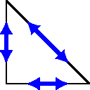
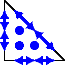
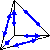
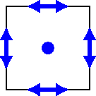
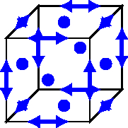
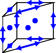
The canonical Regge interpolant \(\mathcal{I}_{Reg}^k\) is defined by the requirement to preserve tangential-tangential moments at edges and inner moments
and can easily be extended to higher dimensions.
Further applications of Regge finite elements
Besides their essential contribution in discretizing the metric tensor of (pseudo-)Riemannian manifolds for curvature approximation and numerical relativity, Regge finite elements have been successfully used to discretize fields in elasticity.
Avoiding membrane locking in (nonlinear) shell analysis by interpolating the membrane stresses into the Regge finite element space Neunteufel, Schöberl. Avoiding membrane locking with Regge interpolation. Computer Methods in Applied Mechanics and Engineering, (2021).
Linear and nonlinear elasticity (continuum mechanics) by discretizing the strain/stress tensor by Regge elements Li. Regge Finite Elements with Applications in Solid Mechanics and Relativity. PhD thesis, (2018)., Hauret, Hecht. A discrete differential sequence for elasticity based upon continuous displacements. SIAM Journal on Scientific Computing, (2013)., Neunteufel, Pechstein, Schöberl. Three-field mixed finite element methods for nonlinear elasticity. Computer Methods in Applied Mechanics and Engineering, (2021).